Survival Analysis of Randomized Placebo-controlled Trial of HIV-1 disease
1.TL;DR
In this analysis, survival Cox-ph model shows that portential risk factors for HIV-1 includes whether or not patients receive previous treatments (tx), patients’ ability to tolerate chemotherapy (karnof) and patient’s baseline cd4 counts (cd4). Exploratory analysis on mean, median survival time for HIV patients and non patients were compared before performing the model. This is the analysis I did when I took Survival Analysis course (BST 222) at UC Davis.
2.Introduction
HIV (human immunodeficiency virus) is a virus which attacks human immune system. People can get infected through the transfer of blood, breast milk, etc. Between the two types of HIV, HIV-1 is more virulent, which can cause infections globally. Zidovudine was the first drug approved by FDA for treatment of HIV infection. However, the survival benefit of the zidovudine-monotherapy only lasts for several months. In the late 1990s, people found that HIV- protease inhibitor could prevent the maturation of virions. Therefore, researchers started to try combination therapy of three drugs which includes a potent HIV-protease inhibitor indinavir (IDV) and two nucleoside analogues lamivudine (3TC) and zidovudine (ZDV) or stravudine (d4T). The goal of this analysis is to build a Cox-ph model and to compare the survival time with or without IDV using the AIDs clinical trial group study 320 data. The descriptions of the data are in Appendix I. The data is a record of 1151 HIV-I patients.
3.Methods and Results
For knowing more about the survival distributions, survival function and hazard function were computed. The data contains 1151 patients who were randomly received one either treatment with IDV or treatment without IDV. The event of interest in this study was patients whose disease progressed to AIDS or death. There are 1055 patients were censored (red dot in Figure 1) and 96 patients were non-censored.
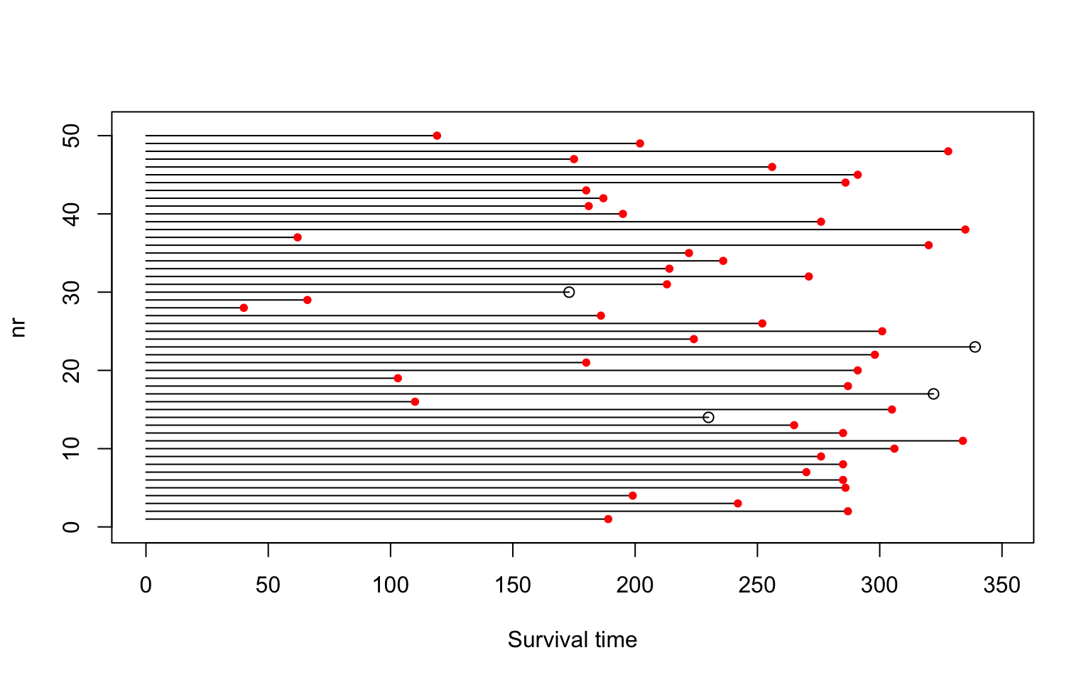
Figure 1: An overview of our data.
a. Survival function
There are two ways to calculate the survival functions. One is to use non-parametric estimator Kaplan-Meier. Another one is to make parametric assumptions and calculate the survival function based on the assumptions, ex: event time follows exponential, Weibull, Gamma, etc.
a1. Kaplan-Meier (nonparametric)
Figure 2 top left shows the estimated survival function with 95% confidence interval band for 1151 patients. Figure 2 top right shows the estimated survival functions separately for treatment group (with IDV) and control group (without IDV). We can see that the proportion surviving of treatment group is longer than the control group. Figure 2 bottom left shows the estimated survival functions for sex. The two survival functions cross each other, which implies their hazards functions are not proportional. Overall, the number of females survive are larger than male. Figure 2 bottom right shows the estimated survival for CD4 groups. We can see that 95% of people with more CD4 cell counts at screening still survive at the end of study. That is because CD4 is an essential part of the human immune system. People who have more CD4 have stronger immune system before doing any treatments. After treatments, the CD4 cell count for all patients increase. So the patients with more CD4 still have stronger defense against virus.
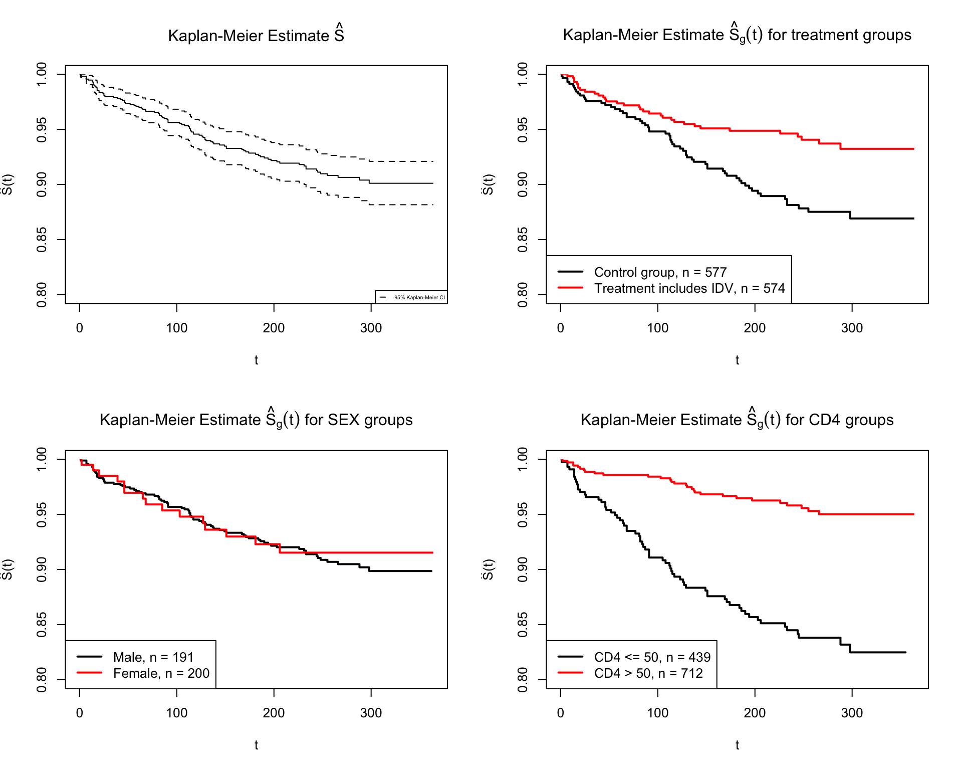
Figure 2: The Kaplan-Meier estimate of survival functions for different groups
a2. Assume exponential distribution, a parametric approach
If we assume the event time follows exponential distribution, the hazard function and survival function are shown as follows.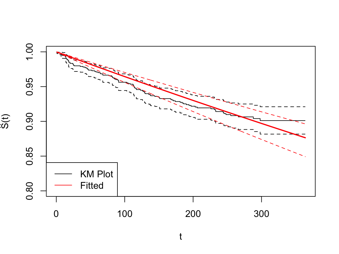
Figure 3: The fitted survival functions for the entire population
b. Mean and Median Survival
The mean survival is the expected value of survival time. The median survival time is defined as the time survival probably is 0.5. The expected mean survival time calculate using Kaplan Meier surviving function is 340.03 with 2.38 standard error. Since the minimum of survival probability is 0.9, it is not possible to reach 0.5 based on our data (Figure 1 topleft). The estimation for median is not available.
S1 = Surv(AIDs$time, AIDs$censor)
fit1 = survfit(Surv(AIDs$time, AIDs$censor)~1, conf.type = "log-log")
print(fit1, print.rmean=TRUE)
## Call: survfit(formula = Surv(AIDs$time, AIDs$censor) ~ 1, conf.type = "log-log")
##
## n events *rmean *se(rmean) median 0.95LCL 0.95UCL
## 1151.00 96.00 340.03 2.38 NA NA NA
## * restricted mean with upper limit = 364c. Compare two models
From Figure 4, we can see there is a difference between treatment group (with IDX) and the control group (without IDX). However, we should compute a test statistic from the observed data to see if they are statistically different.
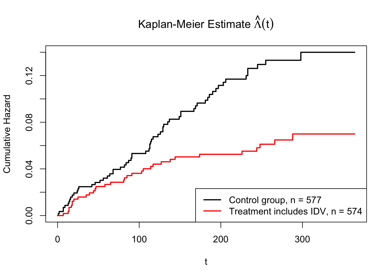
Figure 4: The Nelson-Estimate for accumulative hazard based on two treatments
The sum of those chi-square statistics is 24.47421. And this follows \(\chi^2_7\). The critical value for \(\chi^2_7(0.95) = 14.06714\). The p-value is 0.00094. That means we should reject the null hypothesis and conclude that there is significant difference in survival function/accumulative hazard function between control and treatment group at 0.05 significance level.
d. COXPH model
In order to learn more of the potential risk factors for HIV-1, an initial Cox proportional hazards model is built.
A description of each variable, including description of some key values, is given below.
| Variable Name | Description | Value |
|---|---|---|
| Time | Time to AIDS diagnosis or death | Days |
| Censor | Event indicator for AIDS defining diagnosis or death |
1 = AIDS defining diagnosis or death 0 = Otherwise |
| Tx | Treatment indicator diagnosis or death |
1 = Treatment includes IDV 0 = Control group (treatment regime without IDV) |
| Strat2 | CD4 stratum at screening | 1 = CD4 > 50 0 = CD4 <= 50 |
| Raceth | Race/Ethnicity | 1 = White Non-Hispanic 2 = Black Non-Hispanic 3 = Hispanic (regardless of race) 4 = Asian, Pacific Islander 5 = American Indian, Alaskan Native 6 = Other/unknown |
| Ivdrug | IV drug use history | 1 = Never 2 = Currently 3 = Previously |
| Hemophil | Hemophiliac | 1 = Yes 2 = No |
| Karnof | Karnofsky Performance Scale | 100 = Normal 90 = Normal activity possible 80 = Normal activity with effort 70 = Cares for self; |
| cd4 | Baseline CD4 count | |
| Priorzdv | Months of prior ZDV use | Months |
| age | Age at Enrollment | Years |
Initial model: \[coxph(Surv(time, censor) = factor(tx) + factor(strat2) + factor(raceth) + factor(ivdrug) + factor(hemophil) + factor(karnof) + cd4 + priorzdv + age, data = AIDs)\]
d1. Model Selections
In this analysis, we only consider first order covariates. There is no interactions or higher order terms in the model. Backward selection is applied to the initial model. Among the potential candidates for elimination from the model, the one with the smallest AIC value is the best. The best model from stepAIC command is coxph(Surv(time, censor) ~ factor(tx) + factor(ivdrug) + factor(karnof) + cd4 + age, data = AIDs) The initial model’s AIC is 1238.92. The AIC of this best model is 1228.99. The summary of this model shows that not all the variables’ coefficients are significant at significant level of 0.05. IVdrug (IV drug use history) is not significant with p-value 0.47 and 0.06 (since there are three levels of ivdrug). Age is also not significant with p-value 0.06.
Therefore, the final model is updated to be \[coxph(Surv(time, censor) = factor(tx) + factor(karnof) + cd4, data = AIDs)\]
## Call:
## coxph(formula = Surv(time, censor) ~ factor(tx) + factor(karnof) +
##     cd4, data = AIDs)
##
##   n= 1151, number of events= 96
##
##                        coef exp(coef)  se(coef)      z Pr(>|z|)
## factor(tx)1       -0.646524  0.523863  0.215381 -3.002  0.00268 **
## factor(karnof)80  -0.446976  0.639559  0.364834 -1.225  0.22052
## factor(karnof)90  -1.142121  0.319141  0.360471 -3.168  0.00153 **
## factor(karnof)100 -1.589237  0.204081  0.404259 -3.931 8.45e-05 ***
## cd4               -0.014031  0.986066  0.002492 -5.631 1.80e-08 ***
## ---
## Signif. codes:  0 '***' 0.001 '**' 0.01 '*' 0.05 '.' 0.1 ' ' 1
##
##                   exp(coef) exp(-coef) lower .95 upper .95
## factor(tx)1          0.5239      1.909   0.34347    0.7990
## factor(karnof)80     0.6396      1.564   0.31285    1.3075
## factor(karnof)90     0.3191      3.133   0.15745    0.6469
## factor(karnof)100    0.2041      4.900   0.09241    0.4507
## cd4                  0.9861      1.014   0.98126    0.9909
##
## Concordance= 0.777  (se = 0.023 )
## Likelihood ratio test= 95.84  on 5 df,   p=<2e-16
## Wald test            = 79.82  on 5 df,   p=9e-16
## Score (logrank) test = 97.56  on 5 df,   p=<2e-16
d2. Model Diagnostics
- Assessing Goodness of fit using Martingale Residuals The importance of a good model is its ability to accurately predict the result. Martingale residuals measures the difference between the observed censoring value (0 or 1) and the expected censoring value under a particular Cox model. If the model is correct, the Margingale residuals are distributed with expected value 0. Therefore, by plotting the Martingale residuals of final model against each covariate, we can see to the distribution of those residuals with under different values of covariates in 5. For continuous variable cd4, non-parametric LOESS-smoother with its 95% confidence intervals is added to the plot. The residuals versus all covariates are evenly distributed. There are some outliers in each covariate. But it is improved compared to the null model.
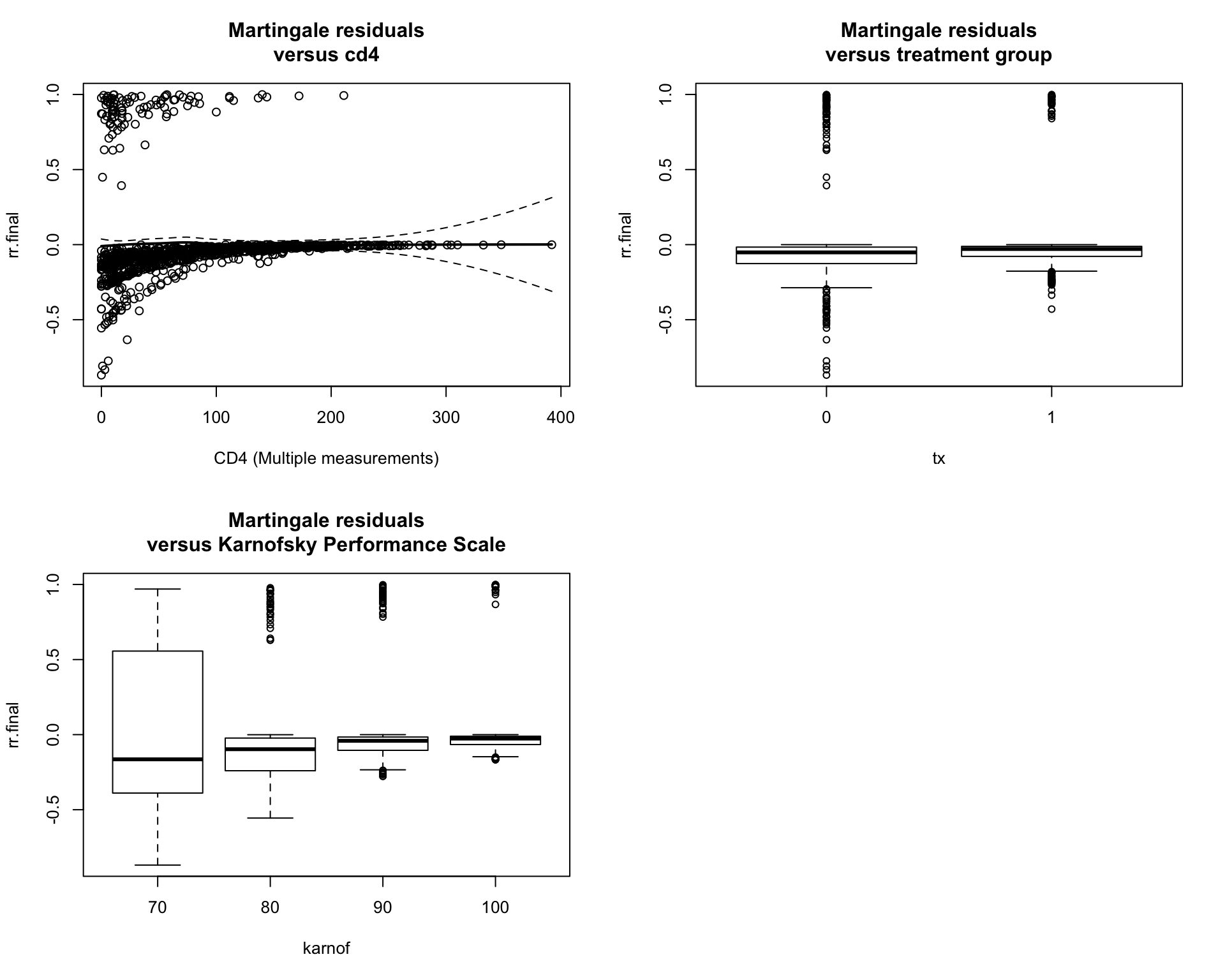
Figure 5: The Martingale residuals against each covariate
- Checking the proportion hazards assumption The proportion hazards are the key assumption in the Cox model. It allows us to cancel out the baseline hazard. If a categorical variable with many levels has a parallel log hazard functions. The proportion hazards assumption holds. Therefore, the log cumulative hazard plots are drawn here 6. As you can see, the categorical variables have a parallel log hazard function. Therefore, this assumption holds for this model.
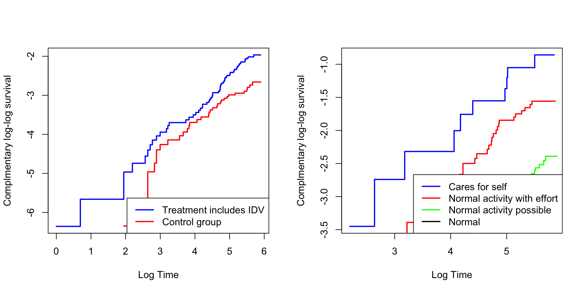
Figure 6: The proportional hazard for treatment and karnofsky performance scale
- Checking the proportion hazards assumption using Schoenfeld residuals Testing the time dependent covariates is equivalent to testing for a non-zero slope in a generalized linear regression of the scaled Schoenfeld residuals on functions of time. Therefore, by using zph function, I can calculate the scaled Schoenfeld residuals directly. A non-zero slop is an indication of a violation of the proportional hazard assumption. As shown in Figure 7, almost all the predictors has all zero slope. Therefore, we can keep all the predictors in the model.
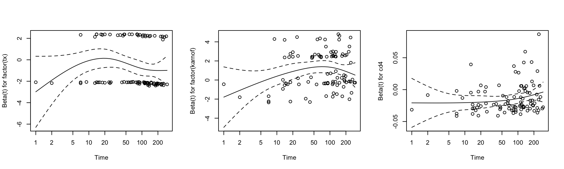
Figure 7: Schoenfeld residuals plot
- Goodness-of-fit test if the model follows exponential (1) distribution
Then the Kolmogorov-Smirnov test is used to test if the model follows exponential one distribution. And the p-value for this test is < 2.2e-16, meaning it does not follow exponential one distribution.
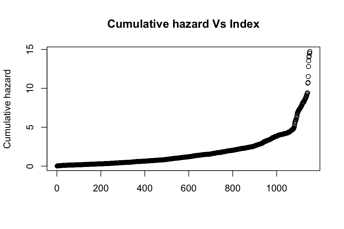
Figure 8: Check if cumulative hazard follows exponential one